Georg Hosoya

In one of my last posts I hinted to the fact that JAGS could be used for simulation studies. Let’s have a look! So basically simulation studies are very useful if one wants to check if a model one is developing makes sense. The main aim is to assess, if the parameters one has plugged into a data simulation process based on the model could be reasonably recovered by an estimation process. In JAGS it is possible to simulate data given a model and a set of known parameters and to estimate the parameters given the model and the simulated data set. For today’s example I have chosen a simple psychometric latent variable measurement model from classical test theory, which is very well understood and can be easily estimated with most software capable of latent variable modeling. Here it is:

$\mu_{1i}=\lambda_1\cdot\eta_i+\beta_1$
$\mu_{2i}=\lambda_2\cdot\eta_i+\beta_2$
$\mu_{3i}= 1\cdot\eta_i+\beta_3$ .

$y_{1i} \sim \mbox{dnorm} (\mu_{1i}, \sigma^2_{e1})$
$y_{2i} \sim \mbox{dnorm} (\mu_{2i}, \sigma^2_{e2})$
$y_{3i} \sim \mbox{dnorm} (\mu_{3i}, \sigma^2_{e3})$

$\eta_i \sim \mbox{dnorm} (0, \sigma^2_{\eta})$

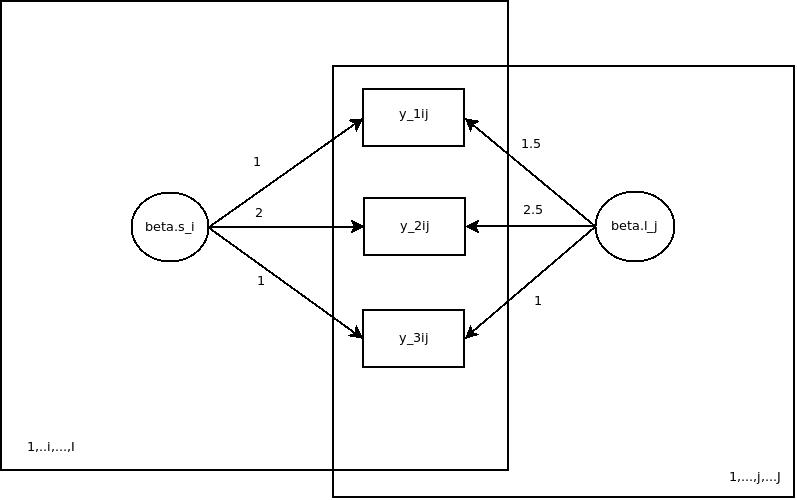
The basic idea is that a latent trait $\eta$ is measured by three items ( $y_{1i}$ to $y_{3i}$ ) with different difficulties ( $\beta_1$ to $\beta_3)$ , different loadings ( $\lambda_1$ and $\lambda_2$ ) and different measurement error variances ( $\sigma^2_{e1}$ to $\sigma^2_{e3}$ ). For identification reasons, the loading of item 3 is set to 1. Furher the variance of the trait ( $\sigma^2_{\eta}$ ) has to be estimated from data.

For simulating data with JAGs we have to specify a data block. The model specification is straight forward, note that we have to hand over the true parameters to JAGS, for example with an R script. This is pretty handy because one could design a thorough simulation study for different sample size and parameter combinations. The estimation part has to be specfied in a model block.

#Simulation
data{
 
  for(i in 1:n)
  {
      y1[i]~dnorm(mu1.true[i], tau.y1.true);
      y2[i]~dnorm(mu2.true[i], tau.y2.true);
      y3[i]~dnorm(mu3.true[i], tau.y3.true);
 
      mu1.true[i]<-lambda1.true*eta.true[i]+beta1.true
      mu2.true[i]<-lambda2.true*eta.true[i]+beta2.true
      mu3.true[i]<-eta.true[i]+beta3.true
  }
 
  tau.y1.true<-pow(sigma.y1.true, -2); 
  tau.y2.true<-pow(sigma.y2.true, -2);
  tau.y3.true<-pow(sigma.y3.true, -2);
 
}
 
# Estimation
model{
 
  for(i in 1:n)
  {
    y1[i]~dnorm(mu1[i], tau.y1);
    y2[i]~dnorm(mu2[i], tau.y2);
    y3[i]~dnorm(mu3[i], tau.y3);
 
    mu1[i]<-lambda1*eta[i]+beta1
    mu2[i]<-lambda2*eta[i]+beta2
    mu3[i]<-eta[i]+beta3
  }
 
  for(i in 1:n)
  {
    eta[i]~dnorm(0,tau.eta);
  }
 
  # Priors for the loadings
  lambda1~dnorm(0,1.0E-3)
  lambda2~dnorm(0,1.0E-3)
  bias_lambda1<-lambda1-lambda1.true
 
  # Priors for the easiness parameters
  beta1~dnorm(0,1.0E-3)
  beta2~dnorm(0,1.0E-3)
  beta3~dnorm(0,1.0E-3)
  bias_beta1<-beta1-beta1.true
 
  # Hyperprior for latent trait distribution
  tau.eta<-pow(sigma.eta,-2)
  sigma.eta~dunif(0,10) 
 
  # Priors for the measurement errors
   tau.y1<-pow(sigma.y1, -2); 
   tau.y2<-pow(sigma.y2, -2);
   tau.y3<-pow(sigma.y3, -2);
   sigma.y1~dunif(0,10);
   sigma.y2~dunif(0,10); 
   sigma.y3~dunif(0,10); 
}

This may look a bit daunting, but it really took only 15 minutes to set that up.

The simulation is controlled by an R script, which hands over the true parameters to JAGS:

library(R2jags)
library(mcmcplots)
 
n=500 # number of subjects
 
# generate 'true' latent trait values
eta.true<-rnorm(n, 0, 4)
# generate 'true' factor loadings
lambda1.true=1
lambda2.true=0.5
 
beta1.true=1
beta2.true=2
beta3.true=3
 
# generate 'true' error standard deviations
sigma.y1.true=1
sigma.y2.true=0.5
sigma.y3.true=0.75
 
data<-list("n", "eta.true", "lambda1.true", "lambda2.true", "sigma.y1.true", "sigma.y2.true", "sigma.y3.true",
           "beta1.true", "beta2.true", "beta3.true")
 
parameters<-c("lambda1","lambda2", "sigma.eta", "sigma.y1", "sigma.y2", "sigma.y3", 
              "beta1", "beta2", "beta3", "bias_beta1")
 
output<-jags.parallel(data, inits= NULL, parameters, model.file="simple_1f.txt",n.chains=2, n.iter=35000, n.burnin=30000)
attach.jags(output)
denplot(output)
traplot(output)
plot(output)

If we inspect the posterior densities based on one dataset with sample size 500 we see that we pretty much hit the spot. That is, all posterior densities are covering the generating true parameters.

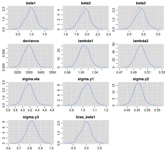
Please note that in the estimation code a posterior density for the difference between the data generating parameter $\beta_1$ and its’ samples from the posterior is specified. The zero is very well covered, but keep in mind that this is based only on one dataset. To replicate a more traditional approach to bias, a viable route could be to simulate several hundreds of datasets and to record for example the posterior mean for each parameter and data set to assess bias.

As always, keep in mind that this is pretty experimental code and estimating latent variable models with JAGS is not very well explored yet as far as I know. However, the main point of this post was to show how JAGS could be used in combination with R to run simulation studies in a probabilistic graphical framework. Should work for multilevel models or generalized mixed models too.

Edit: I just stumbled about this recent blog post by Robert Grand. So stan should work too. Interesting!

Bayesian estimation techniques were added to Mplus version 7 some time ago. Of course I was interested if MPlus and JAGS come to comparable results when let loose on data. 😉

In particular I was interested in the crossclassified module of MPlus, so I wrote some code to simulate data with R and subsequently recovered the parameters with JAGS and MPlus. Recently I found out how JAGS could also be used as a data simulator for simulation studies, but this is a different topic.

So graphically, the model I used for simulation looks like this:

I have omitted the level-1 residual variances and the variances of the latent distributions in the figure for simplicity reasons. The full model specifications can be gleaned from the source code attached to this post.

To make a long story shot: both approaches, JAGs and MPlus, pleasently come to very comparable results with regard to the parameters. At the moment I am too busy with other things to harp on this more, but I thought it is useful to put the code on the blog in case someone is interested to work on a similar topic in more detail. Thanks to Mr Asparouhov for clarifying some questions with regard to MPlus.

The files:
test.R: code to simulate data from the model, recover the parameters with JAGs, also a bit of convergence diagnostics

test.txt: JAGs model file

cc.inp: MPlus input file

cc.dat: Simulated data. Will be overwritten once the simulation part of test.R is executed.

Get the files here. The code is not very polished but should give an idea how to specify the model in MPlus and JAGs.

personal blog

Wow, I have a blog?

JAGS as a tool for simulation studies

Pictures!

Bayesian estimation with JAGS and MPlus: a quick practical comparison